General site information and help
Information on topics raised in portable-antennas.com site.
About the designers
Each of the antenna designers in this site share a common structure and form, while presenting combinations of controls specific to the type of antenna covered.
In each case, the user is presented with a group of controls in the upper left portion of the page: these controls enable the
user to completely specify the characteristics of the antenna, namely frequency, wire lengths, angles, and so on.
Several of the controls are provided with an "Info" graphic
which, when hovered by the mouse, will display helpful notes and hints on that particular control and its function.
Please note that all length dimensions in this website are given, and calculated,
in meters
(see note below).
Upper left-hand side of each designer
Here are two examples of such groups of antenna design controls, the first from the Linked Dipole designer page, and the second from the OCFD (Off-Center Fed Dipole) designer:
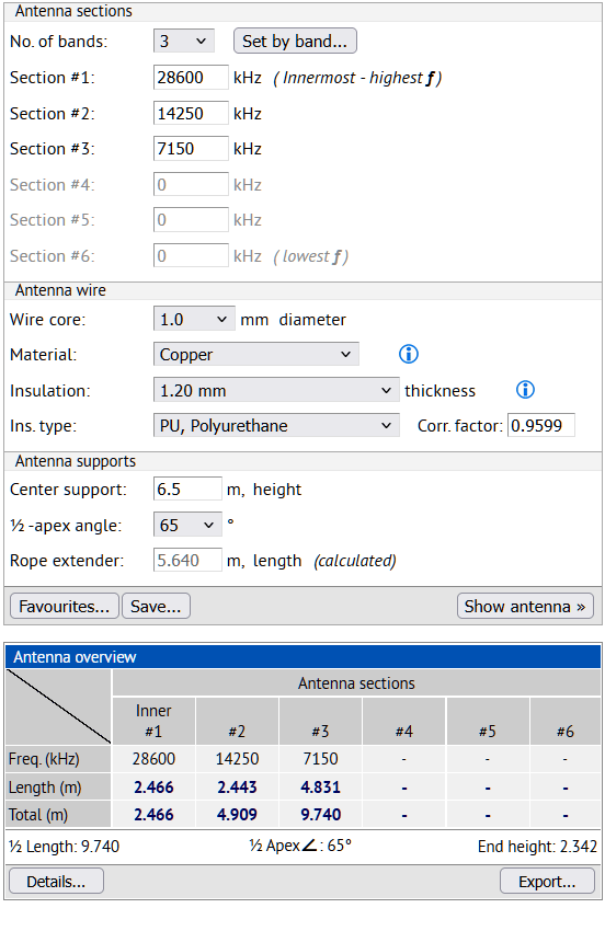
|
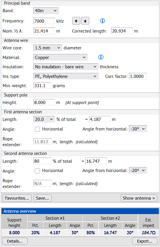
|
| Antenna design controls - Linked Dipole page | Antenna design controls - OCFD page |
Such groups of controls, in each of the antenna designer pages, are similar in style and construction: each set of controls permit entry or choice of parameters specific to the antenna being designed. In each case, the following may be chosen:
- a frequency band or bands, and some means by which the design frequency may be altered;
- configurations specific to the antenna type;
- wire type, size and insulation material and thickness;
- certain dimensions, angles and heights AGL;
- possibly radials, inductors and/or loading coil;
- a button titled " Show antenna "
- a table titled "Antenna overview" listing calculated antenna dimensions.
It's important to note that the design frequency is a frequency which is used by the program to make an initial estimate of the principal dimensions of the antenna, based on electrical principles and physics. This design frequency is NOT the same as the final resonant frequency (the operating frequency) of the physical antenna when built; it's simply used as a parameter to help the program to make as close an estimate of the antenna's dimensions as is possible in the early stages of designing your antenna. You will use the VSWR chart later to make your own estimate of how much the design frequency should be altered in order to achieve the best results at the desired operating frequency of your antenna.
The Show antenna button in this group is very important here, and is the switch which tells the program to calculate, or re-calculate, the physical antenna dimensions for you. Remember, the design philosophy behind the antenna designers in this site is that the user does not have to calculate the physical antenna dimensions: this is all done for you, so that you can concentrate on the shape and disposition of the antenna as it will be, once it has been erected in the field.
Each time you change a setting, or a configuration variable, or height or angle, etc. - you must activate the Show antenna button again, in order to propagate the new settings to the program. If you forget to do this, the program will not be able to present you with the most up-to-date results. Similarly, changes you make to the antenna configuration must be propagated to any radiation patterns, VSWR chart and other diagrams you may have chosen (available further down in the page) by activating the "Display plots" button.
This set of controls also features the following:
- a "Favourites" button (not always available) for managing user-defined antenna configurations for later use;
- a "Save" button (not always available) to save the present configuration to the list of favourites;
- a "Details" button to display a list of antenna sections' lengths and coordinates - useful for comparing results from this program with those from other antenna modelling software;
- an "Export" button to produce an export file (currently limited to PDF) of the main dimensions of the present configuration of your antenna, together with any radiation patterns and other performance charts you may wish to have included.
Upper right-hand side of each designer
In the upper right portion of the page is a graphics area where the modelled antenna is presented in an interactive 3D context. The graphic supports zooming, panning and rotation of the figure. Antenna feed-points are shown as colored markers; the user may also choose to toggle the appearance of a semi-transparent plane at the height (1.76 meters) of an average person, plus an outline human figure, in order to gain some perspective on how large the antenna would appear when erected.
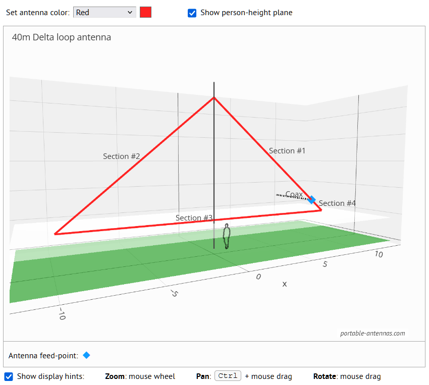
In order to change your viewpoint around the antenna in the 3D diagram, you may zoom, pan or rotate the figure: display hints are provided, showing how this is done using the mouse.
This 3D view of the antenna is refreshed each time the "Show antenna" button is activated.
Lower half of each designer
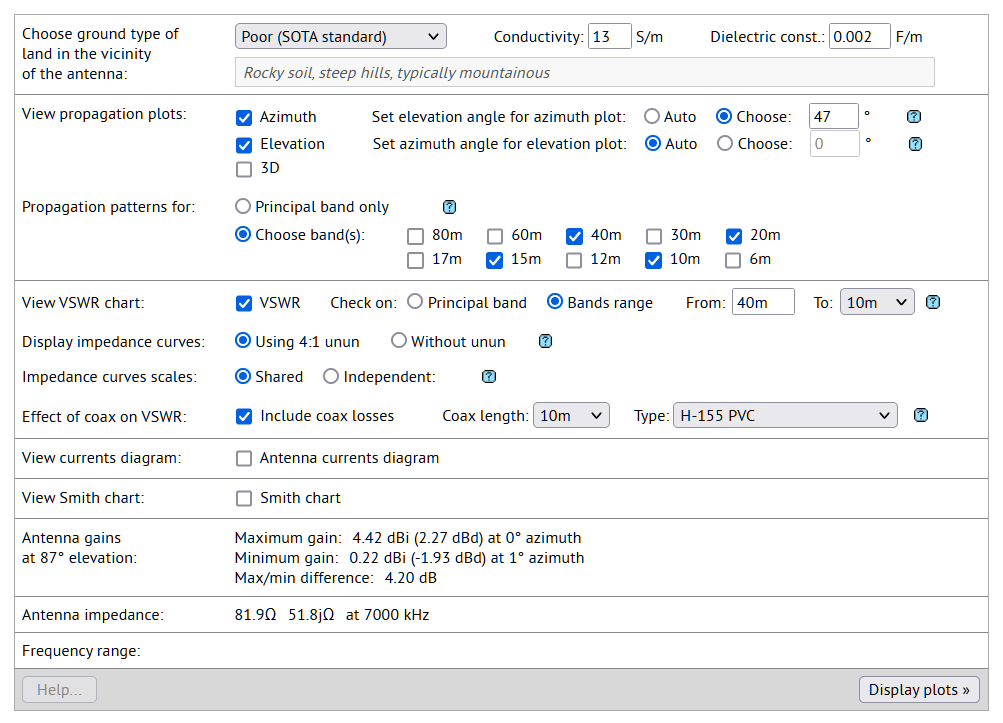
In the lower half of each of the designers, a group of controls enable the calculation of an antenna's performance, and the presentation of charts and diagrams showing the performance in various ways, in any combination of the following:
- azimuth, elevation, 3D and polarization radiation charts
- VSWR charts, incorporating Real- and Imaginary-reactance curves
- an antenna currents diagram
- a Smith chart
Make your choice of applicable ground type, and radiation patterns and other diagrams you wish to generate, together with any additional settings; then activate the "Display plots" button to start the process of calculation and display. Since many of the calculations are performed on the remote server, this can take a little time to complete; results are then returned to your browser for display. Here's an example set of such controls, taken from the OCFD (Off-Center Fed Dipole) designer page:
Calculation of an antenna's performance is achieved using a NEC4.2 (Numerical Electromagnetics Code v4.2) code-base licensed to the site. Results of the calculations, and the resulting charts and diagrams, are entirely comparable with those presented by programs such as EZNec, MMANA-GAL or 4nec2, for similar antennas.
Some notes on the radiation patterns
The newer (since August 2026) style of azimuth, elevation and 3D radiation patterns have been designed to be interactive, such that changes to one or the other of the azimuth and elevation patterns can directly affect the appearance of the others. This is done in order to show more information, and to demonstrate to the interested user how each of these is related to the others, a point which is not made often enough in discussions or display of such patterns.
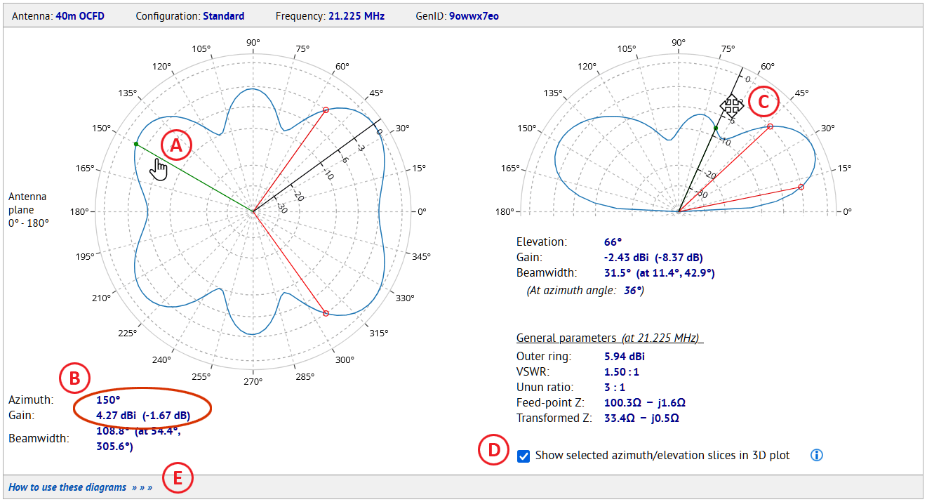
Referring to the two graphics above and below, the user may decide to do one or more of the following:
- hover the mouse Ⓐ over one or the other of the two diagrams to move the green line+marker follower: this will update the display Ⓑ of the angle in the diagram, and the corresponding gain figure;
-
drag the black radial axis Ⓒ to a new position in one or the other of the two
diagrams - this will cause the following changes to occur:
- if the radial axis is moved in the elevation pattern diagram, then the program will calculate a new conical slice Ⓧ at the chosen elevation angle to be taken through the 3D radiation pattern's data, and the azimuth pattern will be updated to reflect the new elevation angle slice;
- if the radial axis is moved in the azimuth pattern diagram, then the program will calculate a new vertical plane slice Ⓨ at the chosen azimuth angle to be taken through the 3D radiation pattern's data, and the elevation pattern will be updated to reflect the new azimuth angle slice.
-
If the "Show selected azimuth/elevation slices in 3D plot" checkbox Ⓓ
has been activated, the 3D radiation pattern will also be updated to reflect the new slice(s):
By inspecting the 3D figure (rotate and pan the figure) one can see that the intersections (the black curves) of cone Ⓧ and plane Ⓨ with the 3D figure are identical with the azimuth and elevation radiation patterns. Indeed, this is precisely how such radiation patterns are generated. It's here that the true value of the three combined radiation patterns reveals itself.
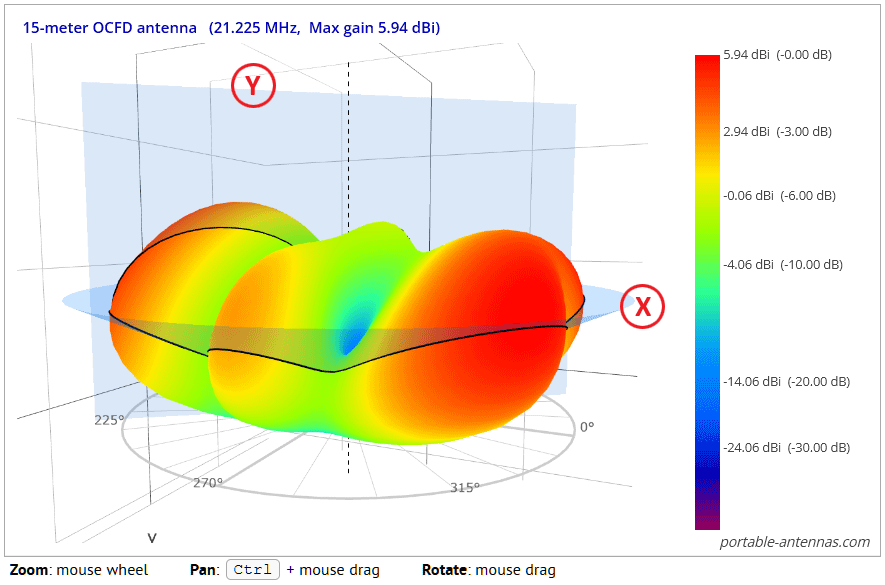 New style 3D radiation pattern
- Activating the "How to use these diagrams" link Ⓔ will display a dialog listing the various levels of interactivity in the three radiation patterns.
Some notes on the VSWR chart
The VSWR chart in the antenna designers in this site can do more than just show a single VSWR curve. In its standard configuration, the chart will display the VSWR curve itself, and also the resistance (real) and reactance (imaginary) components of the antenna's impedance, as functions of frequency.
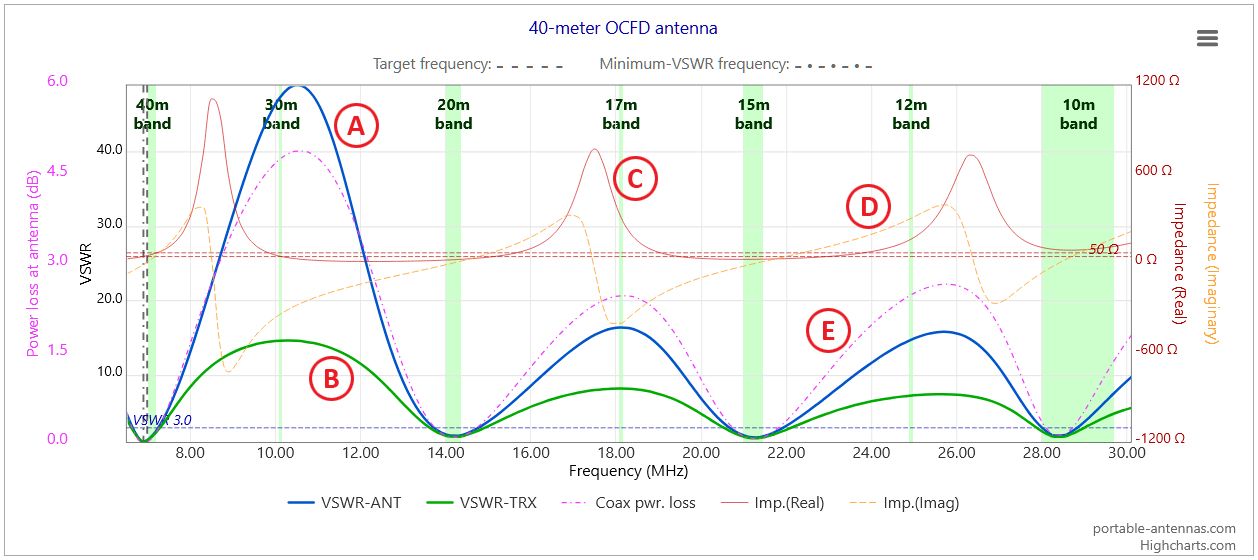
Referring to the above graphic, the user may decide to have the VSWR chart display the following:
- the (blue) VSWR curve Ⓐ (and the resistance Ⓒ and reactance Ⓓ impedance components) for a single band or, if available, for a range of bands - these three curves are standard options;
- by activating the "Include coax losses" checkbox, a second (green) VSWR curve Ⓑ can also be generated, showing the effects, due to attenuation caused by the chosen length and type of coax cable, on the VSWR;
- a power loss curveⒺ, in dB units, will also be displayed, showing how much power is lost in the coax cable, as a function of frequency.
The whole VSWR chart can be zoomed in the X (frequency) direction, so that the user can examine the curve(s) in greater detail. Zooming is achieved by:
- clicking and holding the mouse button down in an area of interest;
- moving the mouse sideways while holding the mouse button down - the area to be zoomed will be highlighted;
- releasing the mouse to complete the action: the chart will now show the zoomed area in expanded form.
- While zoomed-in, the chart can be panned sideways by clicking in the chart while pressing the Shift keyboard key and dragging the chart area left or right.
- To cancel the zoom and return to the default view, activate the "Reset zoom" button which appears in the chart's upper right corner when the chart has been zoomed.
Accuracy of results
Dimensions calculated by our apps and programs most often are accurate enough that the physical antenna, when first erected over suitable ground, will require only minimal trimming to enable it to work at the desired frequency. Nonetheless, NO claims are made concerning the accuracy or applicability of such information; the graphics, data and calculated results presented in this site are provided "as-is" for the general interest and edification of the user. Refer to this site's Disclaimer for more information.
A Note On Length Units
We use meters as length units exclusively and unapologetically throughout this site, since the metric system has been adopted by almost all major industrialized countries in the world. With just one exception - the United States of America, which still uses the cumbersome and outdated Imperial system of measurements which include feet, inches, yards and miles.
Early attempts to include the Imperial system into the calculations, and the display of both metric and Imperial values, in this site indicated very clearly that the additional effort required was just too much, and greatly hindered the further development of the site. With this in mind, and also noting that the entire US population represents less than 4.5% of the world's population, we decided not to support Imperial measurements, and to go forward with metric, the gold standard used by over 95% of the world's population.
Indeed, many US amateurs themselves have decided not to continue to use the Imperial system when designing and building antennas. See e.g. this Youtube video from Toivo W8TJM, where he explains how he has converted completely to metric, "because it's a lot easier to do antenna calculations metrically, rather than trying to convert inches and feet ... none of that conversion's necessary if you go metric."
We have, however, included a metric/Imperial conversion calculator in the Extras page to help those users who may still, in this day and age, be unfamiliar with - or do not yet use - the metric system.
 Web Hosting by Digital Ocean