Radiation patterns - an overview
- An overview of how radiation patterns are generated, and how they relate to each other
- Notes on low-angle antenna radiation and the pseudo-Brewster angle (PBA)
Notes on radiation patterns
Radiation patterns are far-field visualizations, not physical shapes around an antenna. Azimuth, elevation, 3D, and polarization patterns are all derived from the same far-field data, each using a different geometric “slice” through the 3D pattern. Understanding how those slices are defined is essential to interpreting what the plots actually mean.
Key article takeaways » » »
- Radiation patterns describe directional power distribution in the far field, not structures that physically exist around the antenna.
- The NEC modelling software computes gain while assuming far-field conditions (R ≥ 2D²/λ), where pattern shape is independent of distance.
- The 3D radiation pattern contains the full directional information; all other patterns are derived from it.
- Elevation patterns are produced by slicing the 3D pattern with a vertical plane at a chosen azimuth.
- Azimuth patterns are produced by slicing the 3D pattern with a cone at a constant elevation angle—not by a horizontal cut.
- Automatic mode selects azimuth and elevation angles corresponding to maximum gain, but users can override this.
- Polarization plots show horizontal, vertical, and summed components; the summed curve exactly matches the azimuth pattern.
- Antennas at typical portable heights can produce strong vertical polarization in some directions—even for dipole
- Diagrams showing antennas protruding through 3D patterns are schematic, not drawn to scale.
Introduction
Each of the antenna designers in this site allow the user to display one or more radiation patterns:
- an elevation pattern
- an azimuth pattern
- a polarization pattern
- a 3D pattern
For any particular antenna, each of these radiation patterns shows a different aspect of the same thing: namely, how the RF signal energy from the antenna at a particular frequency spreads out, or radiates, from the antenna.
Specifically, the code (NEC v4.2) which generates the gain values used to create these patterns, computes the radiation pattern (gain or directivity vs. azimuth/elevation angles) in the far-field approximation. In this region, the electric and magnetic fields fall off as 1/r, and the angular pattern does not depend on distance (aside from the 1/r amplitude scaling).
The far-field condition - the region around the antenna where the E- and H- fields form radiating waves -
is usually approximated by
R ≳ 2D²/λ
where R = distance from the antenna, D = largest dimension of the antenna, and λ = wavelength.
Hence, for a 20-meter band dipole, this would be greater than a few tens of meters distance from the antenna. The gain values correspond to the normalized power density radiated in a given direction, relative to an isotropic radiator , independent of the observation distance - as long as it's in far-field. This means that, in the far-field region, the radiation pattern is already formed and does not change with distance, unless and until the radiated waves meet an obstruction.
Example - Antenna and the far-field - comparative sizes
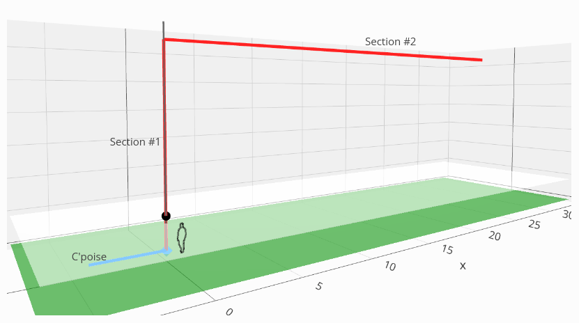
Let's look at an example antenna, an 80-meter EFHW inverted-L, to see how the size of the antenna compares to the size of its radiation patterns. First, the antenna itself:
The azimuth, elevation and 3D patterns for this antenna, on its 6th harmonic at 15 meters, look like this:
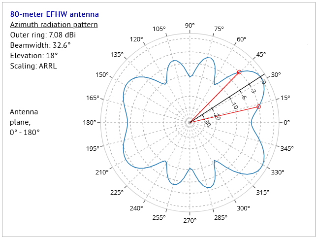
Fig.b - the antenna's azimuth pattern
|
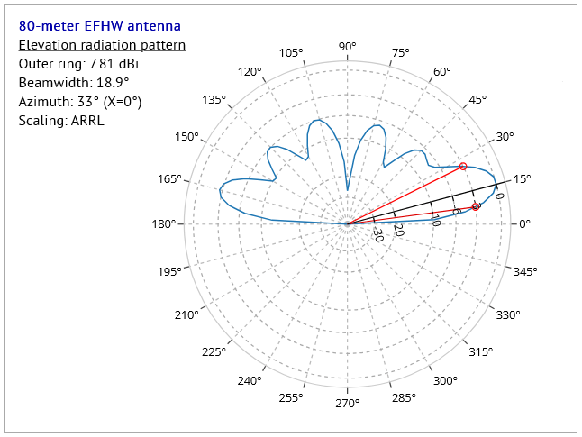
Fig.c - the antenna's elevation pattern
|
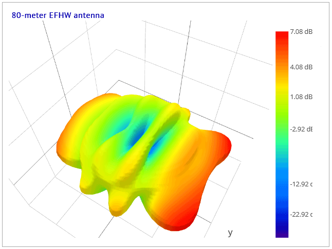
Fig.d - the antenna's 3D pattern
|
Inspecting a larger, and more detailed, version of the elevation pattern as here:
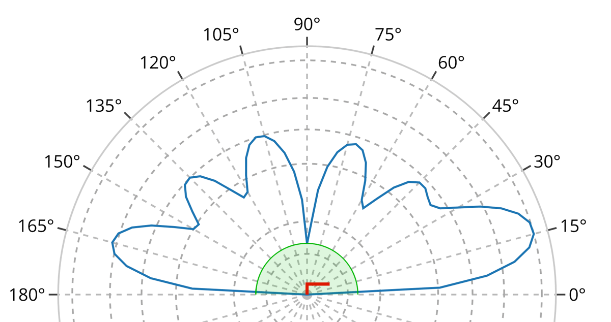
we have included the following elements in Fig. (e), drawn at relative scales intended to illustrate the approximate sizes of the antenna, its far-field region, and its radiation pattern:
- the blue curve represents the elevation radiation pattern of this example 80-meter antenna operating on the 15-meter band (its sixth harmonic);
- the green shaded region represents the minimum distance beyond which the antenna’s far-field region begins and within which a stable radiation pattern cannot yet be defined. On this scale, the green region is shown larger than it would be in reality, in order to make it visible;
- the red inverted-L shape represents the antenna itself. The antenna model is shown slightly enlarged for clarity; at true far-field scale it would often be too small to see!
We should now understand that the radiation pattern - which is defined only at distances greater than approximately
R ≳ 2D²/λ
- exists only in a spatial region (the far field) far larger than the antenna itself, even when depicted (as in Fig. (e)) at the minimum possible distance from
the antenna at which a far-field pattern can be meaningfully defined.
The antenna determines the radiation pattern, but the pattern itself is defined only in the far field as a description of how radiated power varies with direction, rather than as a physical structure surrounding the antenna.
Now, if we inspect radiation patterns from other websites or programs or other publications we may often see graphics like these:
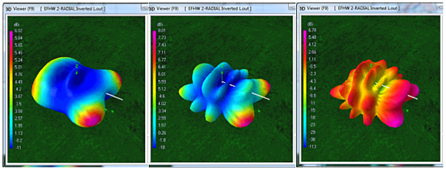
where we can see (as we do in this example produced by the 4NEC2 program) small versions of the antenna (the white lines) protruding from the 3D pattern in certain places.
However, as the far-field relation informs us, the antenna is far smaller than the smallest possible far-field radiation pattern, and hence would never be so large as to be able to protrude anywhere through the 3D pattern surface. We understand such diagrams, therefore, to be representative of the shapes of radiation patterns and their antennas, but to be not representative of their actual sizes.
What the radiation patterns are NOT
First and foremost, the radiation patterns we are familiar with do not actually exist as physical structures anywhere in the real world. There are no corresponding "shapes" to be found in either the electric or magnetic fields of the radiation emitted by an antenna. The forms we see in radiation pattern diagrams are simply conventional visualizations, or graphical encodings, of field strength evaluated at a fixed distance on an imaginary sphere in the antenna's far field.
This particular convention encodes field strength as radial displacement from the center of a polar diagram. Popular usage and long-standing convention often lead us to suppose that the resulting shape somehow exists as a physical structure in space. This is not the case_ the same information could just as easily be encoded in the form using color, shading, contour lines, or as a heatmap, as in this example:

Here we see a "classic" 3D radiation pattern diagram, superimposed on a heatmap representation of the same dataset - each diagram simply presents a different visualization of the same data, namely the RF strength in the RF field at some fixed radius in the antenna's far field.
Either of these visualizations - and many others (see the next section below) - could be used to present this data. However, for consistency and familiarity, we will continue to use conventional radiation pattern diagrams in the discussion that follows, while keeping in mind that they represent only one possible way of visualizing far-field signal strength, rather than any physical structure in the electromagnetic field itself.
"Planetarium-view" 3D radiation pattern
Here we present a special kind of 3D radiation pattern - a so-called "planetarium" view. This displays the radiation gain projected onto a virtual hemispherical "surface" at a constant distance from the antenna - here, an 80m half-square antenna configured as a voltage-fed "EFHW" multi-band antenna, operating on the 10m band. This particular configuration is chosen as a good example displaying several lobes in the pattern, resulting in considerable variation in brightness over the hemisphere.
This kind of view is actually the "true" radiation pattern of an antenna, encoding the radiation gain (as might be measured at many points on the hemispherical surface) as different levels of brightness. The conventional 3D pattern, on the other hand, encodes radiation gain in terms of radius, coupled with color encoding, and is certainly the one we are most familiar with.
Play the video to see this radiation pattern from different elevation angles, starting from a view directly overhead, continuing with decreasing elevation angle, through the horizon, and ending with a view toward the inside of the dome:
(Why "planetarium view?" - well, one could imagine oneself sitting comfortably in a large dome, with a planetarium projector in the center of the dome and, instead of displaying constellations of stars on the inside of the dome, it displays patterns similar to the one in the video.)
The planetarium representation uses a fixed hemispherical dome instead of the conventional 3D radiation envelope. Gain is represented here solely by brightness: brighter regions indicate higher gain in that direction, while darker regions indicate lower gain. The geometry of the dome itself remains fixed, with the radius of the dome depending on the antenna's largest physical dimension and the operating wavelength through the far-field criterion. The dome is often hundreds of meters in radius, with the antenna (at these scales almost invisibly small) at the center.
The One Pattern To Bind Them All - the 3D radiation pattern
It's often assumed by many that the azimuth pattern is simply a "top-view" of the 3D radiation pattern, and that the elevation pattern is the "side-view" of the 3D radiation pattern. We will see, however, that this is not the case, not even in the simplest of examples.
In the following sections, we will attempt to explain how the patterns are generated, how each relates to the others, and to the whole. Some of these relationships are particularly easy to comprehend; others perhaps less so. Let's start with the pattern which shows the most information first: the 3D radiation pattern.
For this discussion, we show a simplified version of a 3D radiation pattern: one for a 40-meter EFHW antenna (a multi-band antenna) being used on one of its resonant bands, the 10-meter band. This antenna is set out in an east-west direction, so that the antenna wires are in the 0° - 180° vertical plane.
We have replaced the usual color information (which would normally be used to show the signal strength at a particular point on the 3D figure) in the 3D patterns diagrams in this discussion, with coloration according to height only, and to highlight certain details in the following sections.
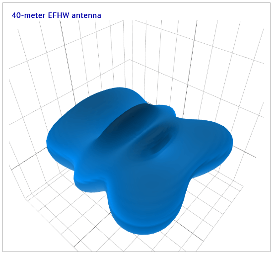
Fig.1 - 3D pattern - basic
|
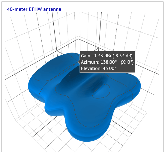
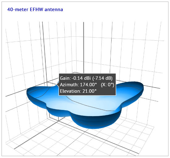
Fig.2 - 3D pattern - basic with tooltip
|
We present here just static images of a 3D pattern, but in a designer page, the 3D figure is capable of being rotated, panned and zoomed. As the second image shows, the figure can also show a tooltip containing information on the point under the mouse pointer.
The azimuth and elevation radiation patterns
The azimuth and elevation radiation patterns each represent "slices" and projections made from the basic 3D pattern for an antenna at a particular frequency. Each of these two patterns is related to the other, with either the program or the user deciding how or where the "slicing" is to take place.
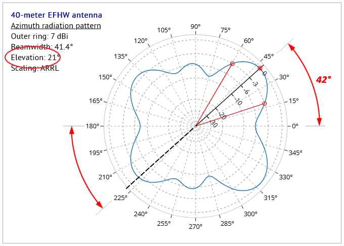
Fig.3 shows an azimuth radiation pattern diagram for this antenna, and we see that the blue outline of the radiation pattern has a shape resembling either a top-down view of the 3D pattern, or a horizontal cross-section through the 3D pattern as displayed in Fig.1 - we will see later that neither of these assumptions in fact represents the true nature of the azimuth pattern. The diagram in Fig.3 is annotated to highlight certain features in the diagram:
- the red dot on the radiation pattern curve represents the maximum gain (7dBi) in the whole pattern - this is at an azimuth angle of 42° from the 0° - 180° line representing the antenna plane;
- the main radial axis (the black line with values 0, -3, -6, -10, etc.) is placed by the program at the angle (42°) of the point of maximum gain;
- for this discussion, we add an extension (the black dashed line) to the radial axis, passing through the diagram center, and out to a point situated diametrically opposite to the point of maximum gain;
- the two lines taken together define the position of the vertical plane used to "slice" through the 3D pattern to produce the elevation pattern in Fig.4.
Here are two views of the 3D pattern after the vertical plane "slice" has been made:
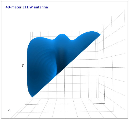
Fig.5 - 3D pattern sliced at 42° azimuth angle, from above
|
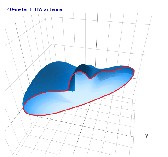
Fig.6 - 3D pattern sliced at 42° azimuth angle, oblique view
|
Note in Fig.6 the outline of the edge (highlighted in red), formed by slicing through the 3D pattern, represents the elevation radiation pattern displayed in Fig.4 above. This demonstrates that an elevation radiation pattern is defined as the profile revealed when the 3D pattern is sliced by a vertical plane aligned along a particular azimuth angle. It's not simply a "side-view" of the 3D pattern.
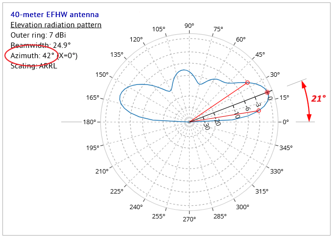
When the program is in "automatic" elevation angle mode - i.e. when the user has NOT chosen a particular elevation angle from the "Choose reference elevation angle" dropdown provided - then the program chooses a point at which BOTH azimuth and elevation angles are set to the angles corresponding to the maximum gain in both azimuth and elevation. Figs. 3 and 4 show the results when the choice is made automatically.
If, however, the user wishes to know what kind of performance the antenna has at an elevation angle OTHER than that chosen automatically by the program, then they can use the "Choose reference elevation angle" dropdown to set this angle manually. Why might the user decide to do this? - reasons for this might include:
- to see how much gain might be got at that angle - the 3D diagram might display a second lobe above the main lobe at a higher angle;
- to compare results between this and other antennas, all at some particular elevation angle, perhaps to see how each compares with the others at an angle suitable for DX;
- because they can, and they're curious to see what the results might be;
...and so on.
Deriving the azimuth radiation pattern from the 3D pattern
Before we go any further, let's see just how the azimuth pattern is obtained from the 3D pattern - it's not an immediately intuitive process, as we hinted at earlier. Let's take a look at the 3D pattern one more time, this time after "slicing" it at a particular elevation angle as chosen either by the program or the user - in this case the elevation angle θ is 21°:
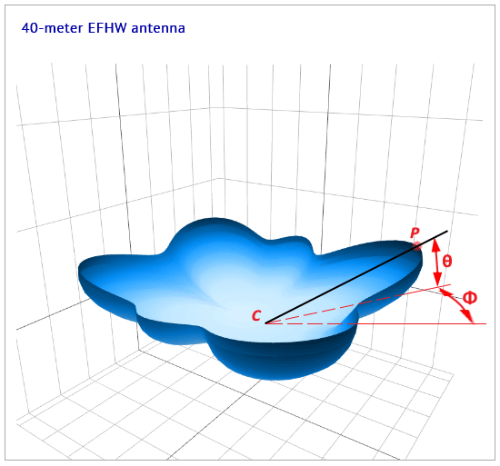
Here, we need to imagine the solid black line, from the antenna center C through the point P on the 3d pattern exterior, as acting like
a rotating knife with its point fixed at the center C, kept at a constant elevation angle θ = 21°, and completing a full 360°
in azimuth Φ. This action describes a cone with apex angle α = 2 × (90°-θ) cutting away the top portion of the 3D pattern, and leaving the bottom portion intact.
The "edge" or "path" revealed, where the 3D pattern has been "cut" or "sliced" in this way, represents the azimuth pattern as shown
in Fig.3 above.
If we were to examine this view of the 3D diagram in the program, we would see that the tooltip shows the elevation angle of 21° at all points along this top edge of the "sliced" diagram, even though this edge looks uneven - it is in fact not at all horizontal! The "slicing" through the 3D figure is not a simple horizontal cross-section of the 3D figure.
Let's now look at a more extreme example: the same antenna, same band, and same 3D pattern as above, but this time with elevation angle set by the user (us!) to a much higher angle of 60°. We use the "Choose reference elevation angle" dropdown to set this angle, and click on the "Display plots" button to show the new azimuth and elevation patterns:
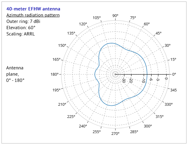
Fig.9 - azimuth pattern, with elevation angle set to 60°
|
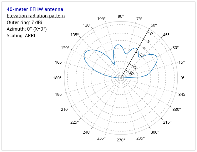
Fig.10 - elevation pattern, with elevation angle set to 60°
|
We see the radial axis in the elevation pattern diagram (Fig.10) set to our choice of 60°, and also that the program has set the azimuth angle to 0°, which just happens to be the direction of maximum gain in this particular configuration.
Looking now at the 3D pattern for this configuration, we see in Fig.11 the 3D pattern sliced at 0° azimuth angle as viewed from the top. In Fig.12, this sliced 3D pattern has been rotated by hand to display an oblique view, where the edge resulting from this slicing has been highlighted in red.
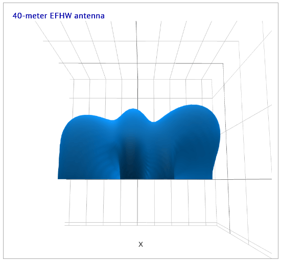
Fig.11 - 3D pattern sliced at 0° azimuth angle, from above
|
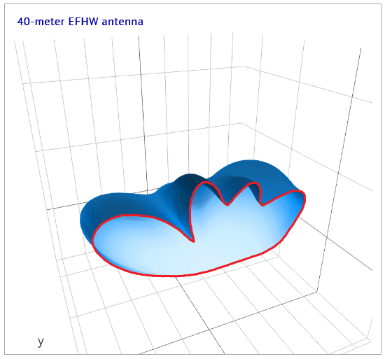
Fig.12 - 3D pattern sliced at 0° azimuth angle, oblique view
|
Again, as in the previous example, the red-highlighted edge reveals the same elevation pattern for this configuration as in Fig.10.
So far, so good - but what about the azimuth pattern in Fig.9? Here we show two views of the 3D pattern after the 60° elevation angle slicing has been applied to it:
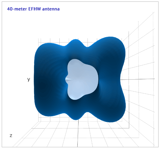
Fig.13 - 3D pattern sliced at 60° elevation angle, from above
|
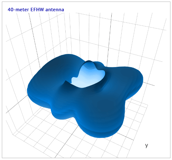
Fig.14 - 3D pattern sliced at 60° elevation angle, oblique view
|
The first figure, Fig.13, reveals the same profile at the cut edge as is displayed in the azimuth radiation pattern Fig.9. The oblique view in Fig.14 shows this profile - produced by an imaginary "knife" set at a constant elevation angle of 60°, and rotated around the center of the antenna - is very far from being a simple horizontal slice through the 3D pattern.
So we see the fundamentally different means by which the azimuth and elevation radiation patterns' profiles are generated:
- azimuth patterns are produced by "slicing" the 3D pattern using a cone described by a line at a constant elevation angle θ, rotated through 360° about the antenna support which is coincident with the Z-axis at the center of the coordinate system used here;
- elevation patterns are produced by "slicing" the 3D pattern using a vertical plane running through the Z-axis of the coordinate system, and at a pre-defined azimuth angle Φ.
Polarization radiation patterns
Polarization radiation patterns are plotted in azimuth, and represent the degree to which the signal is polarized in different azimuthal (compass) directions around the antenna. A single polarization patterns diagram displays three curves at once:
- a vertical polarization pattern,
- a horizontal polarization pattern,
- and a curve representing their summed values,
for a chosen frequency.
So, what is meant by "polarization"? - put simply, it is by convention taken to be the orientation of the electric field (the E-field) of an electromagnetic wave (the RF signal) as it radiates from an antenna; the magnetic field of the wave (the B-field) being here ignored.
Let's take a look at the polarization pattern for the antenna from the previous example, where we chose an elevation angle of 60°:
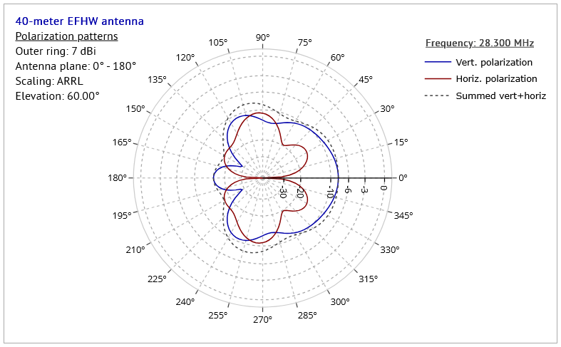
We see in this diagram that the horizontal and vertical polarization patterns have very different shapes, each describing the signal strength in their particular polarization, and in different azimuth (compass) directions around the antenna. The antenna itself is erected in the plane 0° - 180°, i.e. east to west.
In this example, we see that, in directions toward the east (0°) and a little less so toward the west (180°), the vertical component (blue curve) is stronger (> 10dB) than the horizontal; however, in directions orthogonal to the antenna plane, the horizontal component (red curve) wins out, but only just. Those with sharp eyes may already have spotted that the dotted curve representing the combined horizontal and vertical components of the EM field is the exact same shape and size as the azimuth radiation pattern as seen in Fig.9 above. This is, of course, entirely to be expected, since each represents how the whole signal is distributed in azimuth.
Let's take a look at another couple of examples. In the first, we'll look at the polarization patterns diagram for the configuration used for the figure Fig.3 above, where the elevation angle is 21°:
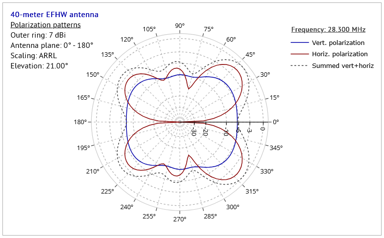
As in the previous example, the vertically polarized component of the radiation is at a maximum in the eastern (0°) and western (180°) directions, but in other directions the situation is mixed, with the horizontal component having several maxima stronger than the vertical. The combined horizontal and vertical components form the dotted "Summed" curve here, which is exactly the same curve as in Fig.3 above.
One more example, this time using a different antenna altogether. Here, we use an inverted-vee dipole for the 20-meter band only, with apex angle of 70° (full apex angle 140°), with the apex at 7m AGL.
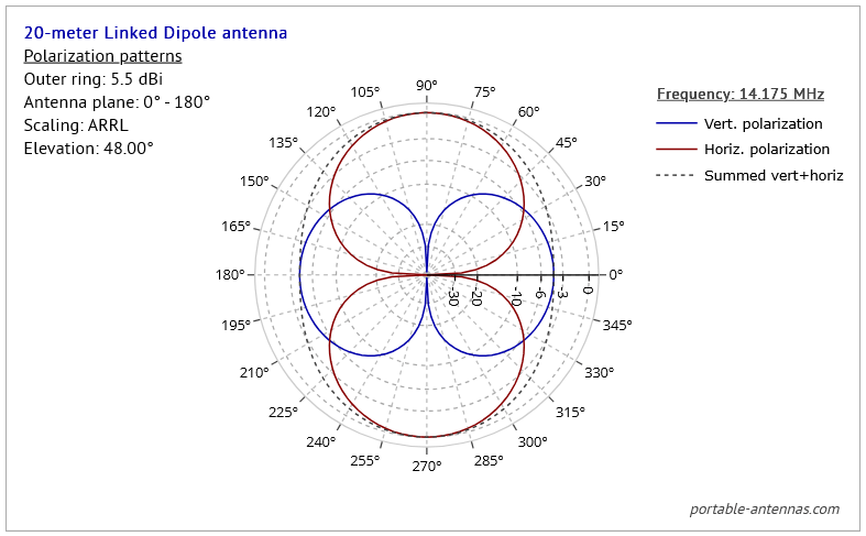
Again, we see the directions of maximum vertical polarization of signal as being along the east-west line, i.e. around the vertical plane of the antenna. But isn't this somehow counter-intuitive? Haven't we all often heard that signals from a dipole are always horizontally polarized, and exclusively so? Indeed, many of us have heard this, but it's a myth - except for dipoles set up VERY FAR above the ground, or situated in "free space."
For dipoles erected at heights AGL typical of portable set-ups - a few meters above the ground - the situation is in fact just as we observe in this example. To get a rough idea of why this would be so, imagine we have set up this antenna on level ground somewhere. We're able to walk around the antenna, viewing it from all azimuth (compass) directions. If we view the antenna from the north or the south (azimuth 90° and 270°) directions, we see the antenna strung out as a long wire as in Fig.17: we would be correct in expecting the signal to be horizontally polarized in these directions, and in directions close to the north-south line.
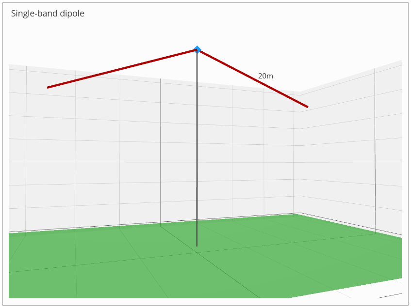
Fig.17 - 20-meter inverted-vee dipole viewed from the side
|
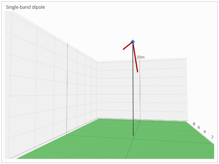
Fig.18 - 20-meter inverted-vee dipole viewed from nearly inline
|
If, however, we walk around the antenna to a position near to the plane of the antenna - i.e. nearly inline with the antenna as portrayed in Fig.18 - the antenna will look very foreshortened, almost like a couple of near-vertical elements. It's in these directions that we observe the maximum vertical polarization from the antenna, almost as if the antenna DID consist of near-vertical elements. Imagining how the antenna looks from different azimuth angles can help us to understand - at least in part - how and why the polarization changes around the compass.
Notes on low-angle radiation and the pseudo-Brewster angle (PBA)
Many users of antenna modelling software assume that the results produced by the software are accurate and dependable under most circumstances. Like all simulations, however, such results should be regarded as representative of an antenna's real-world performance only up to a point. Beyond this point (which cannot be strictly defined), increasing discrepancies between simulated and measured performance should be expected.
This limitation is particularly relevant for vertically-polarized radiation at low elevation angles. In real-world conditions, such waves experience significantly greater attenuation at low angles than is typically predicted by modelling software. This additional attenuation becomes increasingly significant at angles below the so-called pseudo-Brewster angle (PBA), which depends on frequency and the electrical properties of the ground, and rapidly increases as the elevation angle approaches zero.
Key article takeaways » » »
- The pseudo-Brewster angle (PBA) is the elevation angle at which vertically-polarized radiation begins to experience rapidly increasing absorption in the ground rather than reflection.
- The PBA depends primarily on ground dielectric constant, ground conductivity, and frequency.
- For typical HF ground parameters the PBA usually lies in the range of roughly 5° to 10° elevation, although it can be lower over very good ground or seawater.
- Below the PBA, an increasing fraction of the radiated energy is absorbed into the ground instead of being reflected.
- NEC and similar antenna modeling programs do not explicitly track power absorbed in the ground, which can lead to optimistic predictions of gain at very low elevation angles.
- The effect is most important for antennas intended for long-distance (DX) communication, where radiation at very low elevation angles is significant.
- Comparisons between antennas based on modeled gain below the PBA should therefore be treated with caution.
Polarization components
All wire antenna types used in portable operations emit RF waves with horizontal and/or vertical polarization, depending on the azimuthal (compass) direction around the antenna. By convention, polarization is defined by the orientation of the electric field (E-field) of the electromagnetic wave as it propagates away from the antenna; the associated magnetic field (B-field) is not considered here.
Horizontally-polarized radiation, as produced by many types of antenna including dipoles, reflects more strongly from the ground than vertically-polarized radiation, and hence suffers less pseudo-Brewster absorption at low angles. Vertically polarized electric fields can drive conduction currents in the soil much more effectively than horizontal fields; hence, when a vertically polarized wave arrives from the antenna at shallow angles, the ground acts almost like a lossy transmission medium rather than a mirror.
Vertical antennas emit almost exclusively vertically-polarized radiation, with only a very small horizontal component. Other antenna types — including dipoles, EFHWs, and delta loops — generally emit RF waves with mixed polarization, with either the vertical or horizontal component predominating depending on azimuthal (compass) direction.
Antennas which produce significant vertically-polarized radiation in some, or all, azimuthal directions are therefore subject to the low-angle ground-loss effects discussed in the previous section.
Effects of ground on vertical polarization
Real ground is often a complex structure, having layers of different composition and compaction at various locations and depths below the surface; some layers will have greater water content than others, and different amounts of minerals dissolved in the water. Soil can also be very deep in some places, thin in others, and can also contain stones, rocks, organic material and even buried utility pipes and lines. Sometimes, the ground underneath an antenna could have little or no soil, being solid rock or even sand to great depths.
Being such a complex system, it's virtually impossible to assign accurate electrical characteristics to the soil or ground beneath an antenna, unless extensive measurements are made at points around the antenna. For most, this is an impractical solution; hence the common use of "standardized" ground types such as those listed here:
| Relative quality |
Conductivity (S/m) | Permittivity (Dielectric constant) (F/m) |
Surface soil type |
|---|---|---|---|
| Very poor | 0.001 | 5 | Cities, industrial areas |
| Poor to very poor | 0.002 | 10 | Sandy, dry, flat, coastal soils |
| Poor | 0.002 | 13 | Rocky soil, steep hills, typically mountainous |
| Average | 0.005 | 13 | Pastoral, medium hills, and forestation, heavy clay soils |
| Good | 0.01 | 14 | Pastoral, low hills, good soil |
| Very good | 0.0303 | 20 | Pastoral, low hills, rich soil |
| Perfect ground | Infinite | N/A | Perfectly conducting ground (not physically realizable) |
| Fresh water | 0.001 | 80 | Fresh water, lakes |
| Salt water | 5 | 81 | Sea water, low sea beach |
| Free space | N/A | N/A | Free space - antenna is in free space |
Values for soil and water types in this list are selected from the table in the ARRL Antenna Book, 20th Edition, p.3-13.
The values listed are used by all the well-known antenna modeling programs, such as EzNEC, MMANA, 4NEC2, and indeed by this site. This is because the antenna analysis software used by these programs, the NEC engine in its' various versions, uses the conductivity and permittivity values from such lists to calculate the ground reflections of the waves emitted by the antenna.
However, because such ground models are highly simplified, they do not represent the true electrical characteristics of the real soil beneath the antenna. Hence, the NEC-modeled ground interaction - which is good at field addition (direct+reflected), phase effects and pattern shaping - does not explicitly track power absorbed into ground, and especially not for vertically-polarized radiation at low elevation angles.
This leads NEC to produce elevation radiation patterns showing a nice low-angle lobe, reporting reasonable-looking efficiency, but to overestimate radiated power at very low elevation angles for vertically-polarized radiation over real ground. The NEC software assumes that if the radiation is not reflected, then it must have radiated; in reality, some of the power was absorbed by the ground, and was spent in heating the ground beneath the antenna.
Hence, the NEC results are overly optimistic at low elevation angles, especially for vertically-polarized radiation: at elevation angles below ~5°, several dB of additional loss can occur. These losses are worst over ground types like poor ground, dry soil or rocky terrain; losses are correspondingly less over wet ground or salt water (where the effect is much reduced.)
Many users of antenna modeling programs are unaware of this overestimation of radiated power at very low elevation angles, and assume all too often that the elevation patterns produced by them are accurate. Not only that, but many assume that, since such patterns are "accurate" at all elevation angles, results from one antenna can be directly compared with those from another antenna or antenna type. Hence, many users will state with confidence that antenna A is "better" than antenna B, since the gain at some low angle - at 5° say - for antenna A is so many dB greater than the gain for antenna B at the same angle.
Thus, in reality, the users are comparing values from each antenna which have been overestimated, sometimes greatly, by the NEC engine used to produced such results! There are many instances of such comparisons to be found in websites and videos online, with their authors making claims which, on further inspection, turn out to be mostly meaningless.
Effects of ground on elevation radiation patterns - PBA visualized
Let's look at an example of an elevation radiation pattern as produced by the NEC engine used in this website's antenna designers. The pattern is for a 15-meter 1/4-wave vertical with 3 radials at 30° from the horizontal, and with base height of 2 meters AGL.
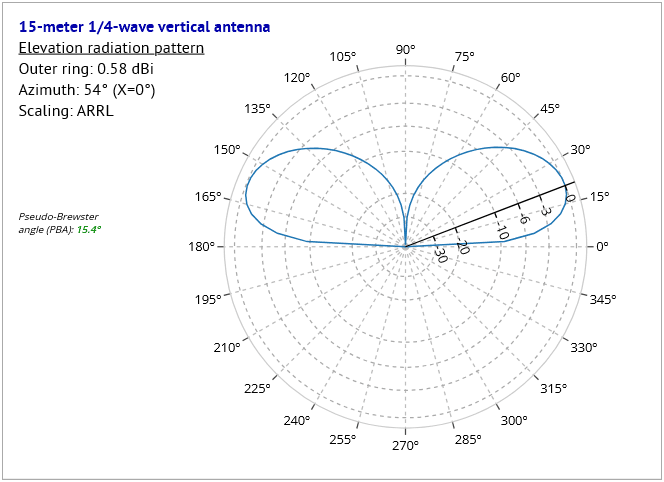
Fig.1 - 15-meter 1/4-wave vertical - elevation pattern
|
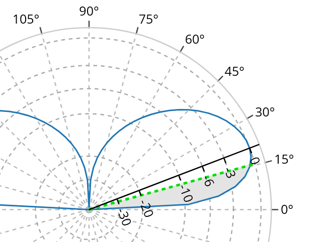
Fig.2 - 15-meter 1/4-wave vertical - elevation pattern detail, showing
pseudo-Brewster angle PBA in green |
In these images, Fig.1 shows the full elevation radiation pattern for the antenna, and Fig.2 shows a detail of the pattern, with additional graphical information. In Fig.2. the green dashed line represents the pseudo-Brewster angle PBA for the frequency (21.0 MHz) and ground type (poor) used in this example; the grey shaded area shows the approximate range of elevation angles below the PBA.
The pseudo-Brewster angle represents the approximate elevation angle below which vertically-polarized radiation begins to suffer rapidly increasing ground absorption rather than reflection.
The PBA itself is calculated with this expression:
where k = the ground dielectric constant, and x = (1.8E4 * G) / frequency, where G = the ground conductivity.
Starting at the PBA, and working down in elevation angle, the program progressively:
- under-estimates ground absorption,
- over-estimates the gain.
Hence at very low angles, the gain figure as reported by the program can be several dB greater than the gain to be expected over real ground. This has real consequences when considering how well a particular antenna may be suited to DX contacts.
Care should be exercised by those seeking to make comparisons with antennas at these low elevation angles!