Use this to chart to estimate additional losses due solely to SWR in a transmission line.

Use this to chart to estimate the SWR at the antenna, given the SWR at the transmitter.

Calculation of losses due to coaxial cable

Real HF transmission lines, in particular coaxial cable, are not perfect conductors of HF energy, and will therefore lead to a certain amount of RF signal loss along their length. Depending on the type and length of transmission line, and the operating frequency, these losses can be quite substantial.

For single-band antennas, such losses are negligible around the resonant frequency. For multi-band antennas - such as OCFD, EFHW antennas, and half-square antennas configured as voltage-fed EFHWs - the losses are also negligible at the various resonant frequencies, but can become very significant at frequencies where the antenna is not resonant:

Fig. 1 - 40-meter EFHW antenna - chart of VSWR at the feed-point

In this example, showing only VSWR values at the antenna feed-point, very high VSWR values are seen at the frequencies where the antenna is not resonant, i.e at the 30m, 17m and 12m bands.

By introducing a configurable length and type of coax cable into the analysis, however, it is possible to transform such high values to ones more accessible to a good antenna tuner:

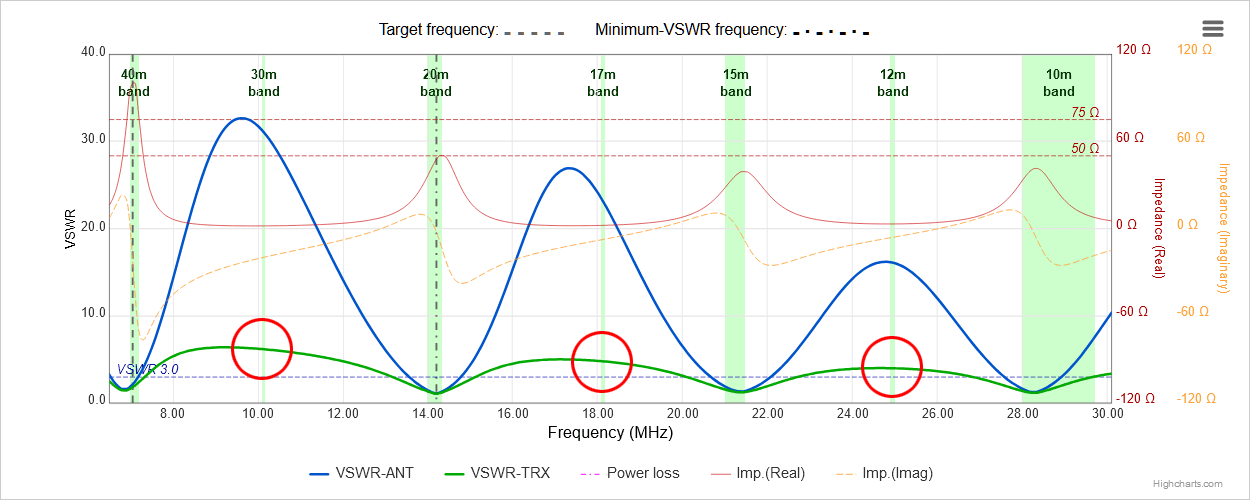
Fig. 2 - 20-meter EFHW antenna - chart of VSWR at feed-point, and at the transmitter end of a length of coax

Here, the green curve shows the VSWR values to be expected at the transmitter end of a length of coax (in this example, 12 meters of RG-316 U coax). It is apparent that the resulting VSWR values at the 30m, 17m and 12m bands are much more amenable to tuning below 3:1 by a decent antenna tuner; it should be understood that this comes at the penalty of higher signal loss.

The following section shows how such losses, and hence VSWR curves at the transmitter end of a length of coax, are calculated.

Estimation of system losses

Losses due to coaxial cable, as mentioned above, can be substantial. Other losses, due to components other than coaxial cable in the transmission system as a whole, can also be significantly high. The various sources of losses which can appear in a typical system are listed here in no particular order:

• Coax / feedline attenuation
  • dependent on cable type, length, frequency, and standing-wave ratio (SWR)
• Transformer/balun/unun losses
  • ferrite core heating
  • winding resistive losses
  • imperfect coupling
  • stray capacitance and leakage inductance
• Antenna conductor losses
  • RF resistive losses in wires, coils, and connections
• Common-mode current suppression losses
  • ferrite chokes, sleeves, or coiled coax ("ugly baluns")
• Ground and environmental losses
  • coupling of RF energy into nearby ground, vegetation, buildings, wiring, or conductive objects
• Matching network / antenna tuner losses
  • resistive and core losses in inductors, capacitors, and transformers

Additionally, losses can arise in the following, if used:

• Loading coil losses
  • especially important in electrically short antennas
• Counterpoise / radial system losses
  • insufficient or lossy return-current paths (very important for EFHWs and portable verticals)
• Connector and junction losses
  • poor connectors, oxidized joints, adapters, and mechanical connections
• Dielectric losses
  • insulation materials, cable dielectrics, traps, coil-formers, and support materials

Any combination of such losses can lead to significant departures from optimal performance of a typical station setup, either portable or at the home QTH.

To see how such losses can affect a typical system of TRX -> coax -> impedance transformer -> antenna, we look first at a typical VSWR chart for, say, a 40-meter EFHW antenna.  This is in and of itself a multiband antenna, and will be resonant on 4 HF bands 40m, 20m, 15m and 10m:

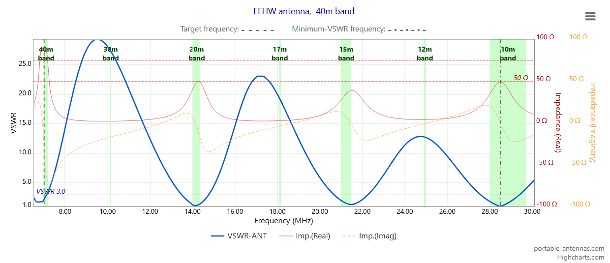
Fig. 3 - 40-meter EFHW antenna - chart of VSWR at the feed-point

This chart shows the VSWR curve for this antenna, at the antenna feed-point: this is the "natural" VSWR curve for such a length of wire (about 20.9m in this case) set up as an inverted-L, and would vary little if the wire type/size/insulation were to be altered, or if the antenna configuration were to be altered slightly.

The points / frequencies of resonance depend almost entirely on the length of wire, and good old text-book physics.  Manufacturers of such EFHW (or OCFD, etc.) antennas may claim their particular choice of wire is the result of much research and analysis of many types of wire, but at the end of the day, their wire is just wire, plain and simple. And wire will produce the kind of curve seen here in Fig.3.

Let's now look at the VSWR curve for this antenna, this time including the (green) VSWR curve to be seen at the TRX end of a length of coax - in this example, we use 16m of RG-58:

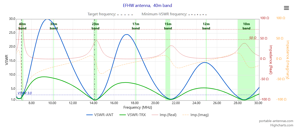
Fig. 4 - 40-meter EFHW antenna - chart of VSWR, including coax losses, at the TRX end of the coax

As we saw in the previous discussion, the coaxial cable has had a profound effect on the "VSWR-TRX" curve shown in green.  This curve shows the VSWR values expected to be seen at the TRX end of this length and type of coax. At the points of resonance, very little difference can be noticed.  At other points/frequencies, however - and especially at the WARC bands 30m, 17m and 12m - the previously very high and unusable VSWR values have been transformed into values more accessible to a very good antenna "tuner."

But this is not the whole story: recall the listing of system losses above which - in addition to those attributable to the coax being used - can also lead to a further diminution of the VSWR curve to be seen/measured at the TRX end of the coax.  Such additional losses can themselves be substantial, enough to lead to an antenna which - if evaluated on the basis of VSWR alone - might be considered to be good, or very good, or even exemplary.

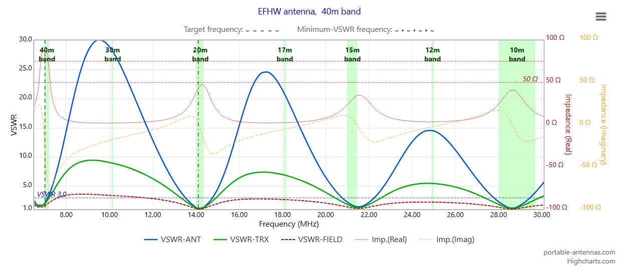
Fig. 5 - 40-meter EFHW antenna - chart of VSWR, including coax and system losses, at the TRX end of the coax

This example (Fig. 5) of the VSWR chart includes these three VSWR curves:

• A standard VSWR curve (blue solid curve)
• VSWR curve after coax losses are included (green solid curve)
• VSWR curve after coax and system losses are included (red dashed curve)

The third curve, which shows the VSWR to be expected at the TRX end of the coaxial cable used in this example, displays usable VSWR values all the way from the 40-meter band up to 10 meters.  We have here used an estimate of the magnitude of the losses to be expected in an average setup of this kind of antenna, evaluated by comparing VSWR curves published by manufacturers of commercial antennas of this type, with the VSWR curves derived by careful NEC modelling of the same antennas.

So, this is a great result, right? - just by including all losses (coax + system) we have an antenna which is eminently usable on all amateur HF bands 40m to 10m: a big win  ...or maybe not...

Remember the "losses" mentioned here and above? - this word is doing a lot of heavy lifting here.  Yes, we may have good, usable VSWR across the bands of interest, but this comes at a cost.  If we inspect a VSWR chart which also includes a curve showing power loss in dB due to coax alone, we can arrive at the cost of including coax losses in the setup:

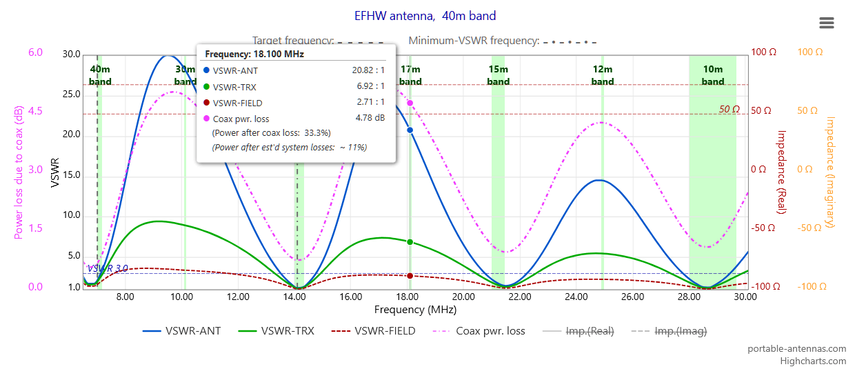
Fig. 6 - 40-meter EFHW antenna - chart of VSWR, including coax and system losses and power-loss curve, at the TRX end of the coax

The power loss curve (magenta dash-dot) shows the true cost to this fairly typical operating setup in terms of power loss in dB.  At points/frequencies of resonance, losses are minimal, around 0.7dB at 40m, up to about 1.1dB at 10m - these values are almost entirely attributable to the losses to be expected from this length and type of caax, and the gentle rise in these values at the resonance minima almost exactly follows the published curve of losses for the coax type.

At other points/frequencies, however - especially at the non-harmonic WARC bands - the magenta curve tells a sobering story of high losses.  Looking at the tooltip featured in the example in Fig. 6, we see that at 17m, the loss in dB is around 4.8 dB, leading to a total power loss of 89%.  That's right - at 17m using this antenna which exhibits fairly typical losses - only about 11% of the signal is actually being transmitted.

But that's the story only for coax losses - the true cost of including coax AND system losses is even more troubling, and can only be estimated / approximated here. Suffice it to say that, if a typical portable station using this antenna setup has 100W TRX output, then at WARC bands, the actual power radiated by the antenna may be as low as 5W or 10W - the rest is lost as heat in the system.  It doesn't really matter if you build your own such antenna, or purchase one from a company making them - the fact of output power loss due to coax+system losses cannot be escaped.

The manufacturers of such wire EFHW/OCFD antennas may be generous enough to publish glowing VSWR charts or numbers for their antennas, but they will never publish figures for the losses to be expected of their antennas.  If they ever did, it's reasonable to imagine many fewer customers would purchase their antennas.